Optimal Power Flow
OPF tries to allocate available generation to meet the current load while keeping transmission lines within the limits of what they can carry. OPF adds a dimension of space to the ED problem. Currently minpower performs the simplest version of power flow, called decoupled OPF and considers only real power 1. The classic text is Bergen & Vittal.
The problem
\(\min \sum_g C_g(P_g)\)
\(\mathrm{s.t.} \; P_{\min (g)} \leq P_g \leq P_{\max (g)} \; \forall \; \mathrm{generators} \;(g)\)
\(\mathrm{s.t.} \; P_{\mathrm{gen} (i)} - P_{\mathrm{load} (i)} - \sum_j P_{ij} = 0 \; \forall \; \mathrm{buses} \;(i)\)
\(\mathrm{s.t.} \; P_{\min (ij)} \leq P_{ij} \leq P_{\max (ij)} \forall \; \mathrm{lines} \;(ij)\)
In this mathematical formulation generators are indexed by \(g\). \(P_g\) is a generator’s power output and \(C_g()\) is its cost function. The objective is to minimize the total cost. There are three constraints:
each generator must be within its real power limits
inflow must equal outflow at each bus
each line must be within its real power limits
For DCOPF, the real power flow on a line \(P_{ij} = \frac{1}{X_{ij}} \left( \theta_i-\theta_j \right)\) depends linearly on the voltage angles of the buses it connects (\(\theta_{i}\), \(\theta_{j}\)) and its own reactance \(X_{ij}\). Bus angles are the difference in voltage angle between the bus and the reference bus which has angle \(0^{\circ}\).
Example Problem
To define a simple OPF problem, Minpower requires three spreadsheets. The first describes the generator parameters and location (generators.csv):
name,bus,cost curve equation
cheap,Tacoma,5P + .01P^2
mid grade,Olympia,7P + .01P^2
expensive,Seattle,10P + .01P^2
The second describes the load at each bus (loads.csv):
name,bus,power
UW,Seattle,50
paper mill,Tacoma,0
smelter,Olympia,50
The third describes the lines between buses (lines.csv):
from bus,to bus,Pmax
Seattle,Tacoma,3
Olympia,Tacoma,10000
Olympia,Seattle,10000
Note
For more information about what options you can specify in each spreadsheet see: Creating a Problem.
Solving
Save the three spreadsheets above into into a folder (call it mypowerflow) and run:
minpower mypowerflow
This particular problem is also Minpower built-in test case, so if you haven’t been following along, to solve it, call:
minpower opf
Example Solution
The result is a plot (powerflow.png):
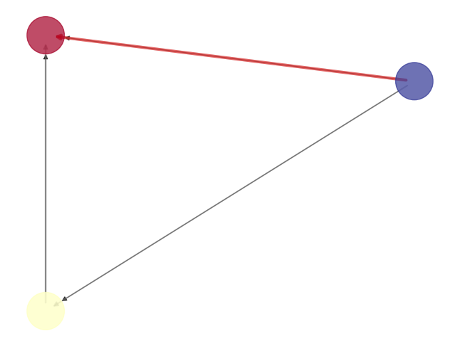
OPF is difficult to visualize (please send suggestions).
A red colored transmission line indicates a limit on that line, while gray lines are below their limits. The Tacoma \(\rightarrow\) Seattle line is at its limit. The other two gray colored lines are running below their limits.
The width of the line indicates the amount of power flow. The Olympia-Seattle line has the largest flow.
The stubs at one end indicate direction of flow. Flow direction is Olympia \(\rightarrow\) Seattle.
Injected power is shown by the color of the bus. Olympia is injecting power into the system while Seattle is pulling power.
There are also spreadsheet outputs of generator information (powerflow-generators.csv):
generator name,u,P,IC
cheap,1,0.0,5.0
mid grade,1,58.9999999999996,8.179999999999993
expensive,1,41.0000000000003,10.820000000000006
and line information (powerflow-lines.csv):
from,to,power,congestion shadow price
Seattle,Tacoma,-3.0,
Olympia,Tacoma,3.00000000000068,
Olympia,Seattle,6.00000000000068,
Each line’s real power flow is output. Lines that have congestion will show a positive shadow price. Because the flow is Tacoma \(\rightarrow\) Seattle and the from/to fields of the spreadsheet are the other way around, we see a negative power flow. The Seattle-Tacoma line is at its limit, so there is an extra cost to the system from the congestion and the line has a positive shadow price.
Footnotes
- 1
Modern power systems often have reactive power issues. While DCOPF is a decent approximate solution with reactive power considered, your results may vary significantly from real operations without it.